Modeling-to-Generate-Alternatives (MGA) Tutorial

MGA is commonly used in energy modelling to address what is known as “structural uncertainty.” That is, the uncertainty stemming from unknown, unmodeled, or unmodel-able objectives. For instance, political feasibility or some other qualitative variable.

The MGA Idea

To get around this challenge, MGA searches the “sub-optimal” or “near-optimal” region for alternative solutions by relaxing the objective function. The goal for a single-objective problem is to find “maximally different solutions in the design space.” In multi-objective problems, specifically ones solved with genetic algorithms, users can identify alternatives by random selection or farthest first traversal.

MGA Example

import numpy as np
import matplotlib.pyplot as plt
import pandas as pd
import itertools as it
# pymoo imports
from pymoo.problems import get_problem
from pymoo.algorithms.moo.nsga2 import NSGA2
from pymoo.optimize import minimize

from osier import n_mga
from osier import distance_matrix, farthest_first, check_if_interior, apply_slack

problem = get_problem("bnh")
seed = 45
pop_size = 100
n_gen = 200
algorithm = NSGA2(pop_size=pop_size)

res = minimize(problem,
               algorithm,
               ('n_gen', n_gen),
               seed=seed,
               verbose=False,
               save_history=True
               )

PF = problem.pareto_front()
F = res.F
a = min(F[:,0])
b = max(F[:,0])
f1 = PF[:,0]
f2 = PF[:,1]
slack = 0.1
alpha = 0.5
F1 = f1 * (1+slack)
F2 = f2 * (1+slack)

X_hist = np.array([history.pop.get("X") for history in res.history]).reshape(n_gen*pop_size,2)
F_hist = np.array([history.pop.get("F") for history in res.history]).reshape(n_gen*pop_size,2)

with plt.style.context('dark_background'):
    fig, ax = plt.subplots(1,2, figsize=(14,6))

    ax[0].set_title("Objective Space")
    ax[0].scatter(F_hist[:,0], F_hist[:,1], facecolor="none", edgecolor="lightgray", label='tested points')
    ax[0].scatter(F[:,0], F[:,1], facecolor="none", edgecolor="red", label='optimal points')
    ax[0].plot(PF[:,0], PF[:,1], color="g", alpha=0.7, label='Pareto front', lw=4)
    ax[0].fill(np.append(f1, F1[::-1]), np.append(f2, F2[::-1]), 'lightgrey', alpha=alpha, label="Near-optimal space")
    ax[0].legend()


    ax[1].set_title("Design Space")
    ax[1].scatter(X_hist[:,0], X_hist[:,1], facecolor="none", edgecolor="lightgray", label='tested points')
    ax[1].scatter(res.X[:,0], res.X[:,1], facecolor="none", edgecolor="blue", label='optimal points')
    ax[1].legend(loc='upper left')
    plt.tight_layout()
    plt.show()

Create the slack front

slack_front = apply_slack(F, slack=slack)

Check for points that are bounded within the Pareto front and the slacked front

int_pts = check_if_interior(points=F_hist, par_front=F, slack_front=slack_front)
X_int = X_hist[int_pts]
F_int = F_hist[int_pts]

Create a distance matrix

This matrix stores the distances from one point to every other point.

D = distance_matrix(X=X_int)

Calculate the farthest points

n_pts = 10
idxs = farthest_first(X=X_int, D=D, n_points=n_pts, seed=seed)

F_select = F_int[idxs]
X_select = X_int[idxs]

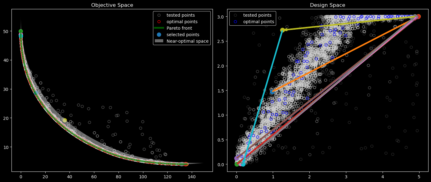
Plot!

The objective space plot (left) shows the selected points in objective space. These points were chosen using a “farthest first traversal” in design space. The design space plot illustrates the path of this traversal.

from mycolorpy import colorlist as mcp
import matplotlib as mpl
import matplotlib.patches as patches

cmap_name = 'tab10'
color1=mcp.gen_color(cmap=cmap_name,n=n_pts)
cmap = plt.get_cmap(cmap_name, n_pts)

with plt.style.context('dark_background'):
    fig, ax = plt.subplots(1,2, figsize=(14,6))

    ax[0].set_title("Objective Space")
    ax[0].scatter(F_hist[:,0], F_hist[:,1], facecolor="none", edgecolor="lightgray", alpha=0.4,label='tested points')
    ax[0].scatter(res.F[:,0], res.F[:,1], facecolor="none", edgecolor="red", label='optimal points')
    ax[0].plot(PF[:,0], PF[:,1], color="g", alpha=0.7, label='Pareto front', lw=4)
    ax[0].scatter(F_select[:,0], F_select[:,1], c=color1, s=80, label='selected points')

    ax[0].fill(np.append(f1, F1[::-1]), np.append(f2, F2[::-1]), 'lightgrey', alpha=alpha, label="Near-optimal space")
    ax[0].legend()


    ax[1].set_title("Design Space")
    ax[1].scatter(X_hist[:,0], X_hist[:,1], facecolor="none", edgecolor="lightgray", alpha=0.2, label='tested points')
    ax[1].scatter(res.X[:,0], res.X[:,1], facecolor="none", edgecolor="blue", label='optimal points')
    ax[1].legend(loc='upper left')

    style = "Simple, tail_width=0.5, head_width=4, head_length=8"
    arrows = []
    prev = X_select[0]
    for i, (c, (x, y)) in enumerate(zip(color1,X_select)):
        ax[1].scatter(x, y, color=c, s=100)
        if i == 0:
            pass
        else:
            kw = dict(arrowstyle=style, color=c, linewidth=3)
            curr = (x,y)
            arrows.append(patches.FancyArrowPatch(prev, curr, **kw))
            prev = curr

    for a in arrows:
        ax[1].add_patch(a)

    plt.tight_layout()
    plt.show()

F_df = pd.DataFrame(dict(zip(['f0','f1'], F_select.T)))
X_df = pd.DataFrame(dict(zip(['x0','x1'], X_select.T)))
mga_df = pd.concat([F_df, X_df], axis=1)

MGA with Osier

The MGA algorithm has several steps. Fortunately, osier offers a self contained function n_mga.

mga_res = n_mga(results_obj=res, slack=slack, seed=seed, wide_form=True)

Confirm that the two methods are equivalent.

mga_df.equals(mga_res)

True