Dispatch Tutorial

In this tutorial you will learn how to run a dispatch model in osier using

1. osier technology objects

2. The osier dispatch algorithm

A dispatch model determines the amount of energy each technology produces at each timestep. This implementation uses a linear program constructed with Pyomo. Since it is a linear program, the model has perfect foresight and minimizes total variable cost.

First, we must import some key ingredients.

# basic imports
import pandas as pd
import matplotlib.pyplot as plt
import numpy as np
from unyt import kW, minute, hour, day, MW
import sys

# osier imports
from osier import DispatchModel, LogicDispatchModel
import osier.tech_library as lib


# automatically set the solver
if "win32" in sys.platform:
    solver = 'cplex'
elif "linux" in sys.platform:
    solver = "cbc"
else:
    solver = "cbc"

print(f"Solver set: {solver}")

Solver set: cbc

Creating the technology portfolio

In order to run a dispatch model you must provide a mix of energy generating technologies. The technologies used in the dispatch model should be added to a python list.

In general, dispatch models do not optimize the capacity of each generator. They only optimize the amount of energy each generator produces (i.e., dispatches).

If you forget what technologies are available in osier (or what they’re called), simply look at the catalog!

lib.catalog()

	Import Name	Technology Name
0	battery	Battery
1	biomass	Biomass
2	coal	Coal_Conv
3	coal_adv	Coal_Adv
4	natural_gas	NaturalGas_Conv
5	natural_gas_adv	NaturalGas_Adv
6	nuclear	Nuclear
7	nuclear_adv	Nuclear_Adv
8	solar	SolarPanel
9	wind	WindTurbine

# create a capacity portfolio of only natural gas.

technology_mix = [lib.natural_gas]
display(technology_mix)

[NaturalGas_Conv: 8375.1331 MW]

Adding energy demand

The other thing a dispatch model needs in order to run is a demand profile to optimize. We will create a dummy demand profile for a 48-hour period for our model to optimize.

n_hours = 24  # hours per day
n_days = 2  # days to model
N = n_hours*n_days  # total number of time steps
phase_shift = 0  # horizontal shift [radians]
base_shift = 2  # vertical shift [units of demand]
hours = np.linspace(0,N,N)
demand = (np.sin((hours*np.pi/n_hours*2+phase_shift))*-1+np.ones(N)*(base_shift+1))

with plt.style.context("dark_background"):
    plt.plot(hours, demand, color='cyan')
    plt.grid(alpha=0.2)
    plt.ylabel('Demand [MW]')
    plt.xlabel('Time [hr]')
    plt.show()

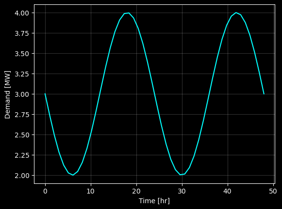
The demand peaks in the afternoon and reaches a minimum around 6 A.M. Although reasonable, we could make it slightly more “realistic” by adding some random noise. We can also adjust curve so the area under the curve matches a known amount of demand.

total_demand = 185  # [MWh], sets the total demand [units of energy]
demand = (np.sin((hours*np.pi/n_hours*2+phase_shift))*-1+np.ones(N)*(base_shift+1))

np.random.seed(1234) # sets the seed for repeatability

noise = np.random.random(N)
demand += noise

demand = demand/demand.sum() * total_demand  # rescale

with plt.style.context("dark_background"):
    plt.plot(hours, demand, color='cyan')
    plt.ylabel('Demand [MW]')
    plt.xlabel('Time [hr]')
    plt.grid(alpha=0.2)
    plt.show()

Creating the Dispatch Model

This is the simplest model in osier. The dispatch model minimizes total operational cost of the system and requires two pieces of data:

1. A list of osier.Technology objects that can meet the specified demand.

2. A net demand profile (i.e., if you want to model renewable energy, you should provide a production curve for the given time period of interest). The net demand is the demand minus the non-dispatchable energy production at each time step (e.g., demand - wind production - solar production).

In order to solve the model, simply call DispatchModel.solve(solver="SOLVER_NAME"). This function returns None, but you can check that it succeeded by printing DispatchModel.objective.

The default values for the model are:

1. Energy – Megawatts [MW]

2. Time – 1 hour [hr]

3. Cost – million dollars per unit [M$/unit]

import time
start = time.perf_counter()
model = DispatchModel(technology_list=technology_mix,
                      net_demand=demand
                     )
model.solve(solver=solver)  # add your preferred solver here!
end = time.perf_counter()
print(model.objective)
print(f"Model ran in {(end-start):3f} seconds.")

0.0041415950022387
Model ran in 0.843126 seconds.

Verifying the results

Since this is only a dispatch model, the only costs that contribute to the merit order is the marginal cost of producing electricity (i.e., the variable costs). Although there are two types of variable costs in an osier.Technology object, fuel and operating and management (O&M). They are automatically combined into a single variable cost (osier tries to enforce consistent units as well by using the unyt library).

In order to verify that the results make sense, we can divide the model objective by the total demand, and that should equal the variable cost for the natural gas technology (though I use the np.isclose command to account for any floating point wonkiness).

tol = 1e-6
np.isclose((model.objective / total_demand),
           model.technology_list[0].variable_cost,
           rtol=tol)

np.True_

The variables agree! Which means the model ran successfully and nothing strange happened!

Checking the results

# show the first 5 hours of the system.
model.results.head()

	NaturalGas_Conv	Curtailment	Cost
0	3.487598	-0.0	0.000078
1	3.669428	-0.0	0.000082
2	3.199753	-0.0	0.000072
3	3.351018	-0.0	0.000075
4	3.172340	-0.0	0.000071

with plt.style.context("dark_background"):
    fig, ax = plt.subplots(figsize=(8,4))
    ax.grid(alpha=0.2)
    ax.minorticks_on()
    ax.fill_between(hours,
                    y1=0,
                    y2=model.results['NaturalGas_Conv'].values,
                    color='tab:orange',
                    label='Natural Gas')
    ax.plot(hours, model.net_demand, color='cyan', label='Net Demand')
    ax.set_xlim(0,48)
    ax.set_ylim(0,5.5)
    ax.legend()
    ax.set_ylabel("Demand [MW]")
    ax.set_xlabel("Time [hr]")
    plt.show()

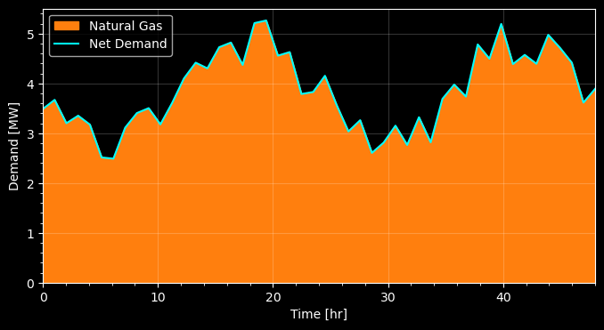
We see that the natural gas plant perfectly fulfilled the demand at each time step.

Hierarchical Dispatch

osier offers a second, faster, dispatch algorithm called osier.LogicDispatchModel. Although this model is faster, it is myopic. Therefore, optimality is not guaranteed. Especially for systems with a lot of renewable energy and battery storage.

LogicDispatchModel can be used as a drop-in replacement for the original DispatchModel.

start = time.perf_counter()
model = LogicDispatchModel(technology_list=technology_mix,
                      net_demand=demand
                     )
model.solve()  # add your preferred solver here!
end = time.perf_counter()
print(model.objective)
print(f"Model ran in {(end-start):3f} seconds.")

0.0041415950000000005
Model ran in 0.101489 seconds.

with plt.style.context("dark_background"):
    fig, ax = plt.subplots(figsize=(8,4))
    ax.grid(alpha=0.2)
    ax.minorticks_on()
    ax.fill_between(hours,
                    y1=0,
                    y2=model.results['NaturalGas_Conv'].values,
                    color='tab:orange',
                    label='Natural Gas')
    ax.plot(hours, model.net_demand, color='cyan', label='Net Demand')
    ax.set_xlim(0,48)
    ax.set_ylim(0,5.5)
    ax.legend()
    ax.set_ylabel("Demand [MW]")
    ax.set_xlabel("Time [hr]")
    plt.show()

Time Benchmarking

%%timeit
model = DispatchModel(technology_list=technology_mix,
                      net_demand=demand
                     )
model.solve(solver=solver)

955 ms ± 118 ms per loop (mean ± std. dev. of 7 runs, 1 loop each)

%%timeit
model = LogicDispatchModel(technology_list=technology_mix,
                      net_demand=demand
                     )
model.solve()

264 ms ± 2.28 ms per loop (mean ± std. dev. of 7 runs, 1 loop each)

We observe almost a 4x speed-up using the LogicDispatchModel over the DispatchModel.