![]()
Capacity Expansion Tutorial#
In this tutorial, we will use osier to optimize the capacity for a test energy system using osier’s CapacityExpansion model.
First we will size a natural gas plant and battery storage for a test system while minimizing total cost.
Next, we will replace the natural gas plant with a wind turbine while still only minimizing for total cost.
Lastly, we reintroduce the natural gas plant and co-optimize two objectives, total cost and lifecycle carbon emissions.
Important Caveat
For simplicity and the sake of time, this notebook specifies a certain number of generations before the model terminates. Therefore it is unlikely that the capacity expansion models shown in this notebook are fully converged. These results should be used for instructional purposes only!
[1]:
# basic imports
import pandas as pd
import matplotlib.pyplot as plt
import numpy as np
from unyt import kW, minute, hour, day, MW
import sys

# osier imports
from osier import CapacityExpansion
import osier.tech_library as lib

# pymoo imports
from pymoo.algorithms.moo.nsga2 import NSGA2
from pymoo.optimize import minimize


# set the solver based on operating system -- assumes glpk or cbc is installed.
if "win32" in sys.platform:
    solver = 'glpk'
elif "linux" in sys.platform:
    solver = "cbc"
else:
    solver = "cbc"

print(f"Solver set: {solver}")
Solver set: cbc
As before, osier needs two fundamental things in order to run the model
A technology set
A net demand profile
Let’s create both of these, first. This time, we’ll also create a dummy “wind” profile and a wind technology to use in the latter two examples. We’ll also borrow some code from the dispatch tutorial.
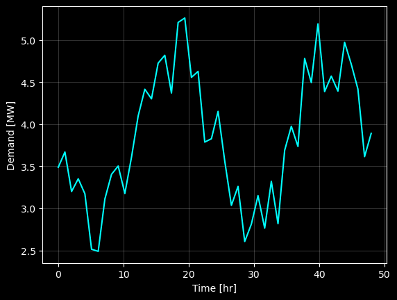
Creating the demand profile#
[3]:
n_hours = 24  # hours per day
n_days = 2  # days to model
N = n_hours*n_days  # total number of time steps
phase_shift = 0  # horizontal shift [radians]
base_shift = 2  # vertical shift [units of demand]
hours = np.linspace(0,N,N)
total_demand = 185  # [MWh], sets the total demand [units of energy]

demand = (np.sin((hours*np.pi/n_hours*2+phase_shift))*-1+np.ones(N)*(base_shift+1))

np.random.seed(1234) # sets the seed for repeatability

noise = np.random.random(N)
demand += noise

demand = demand/demand.sum() * total_demand  # rescale

with plt.style.context("dark_background"):
    plt.plot(hours, demand, color='cyan')
    plt.ylabel('Demand [MW]')
    plt.xlabel('Time [hr]')
    plt.grid(alpha=0.2)
    plt.show()
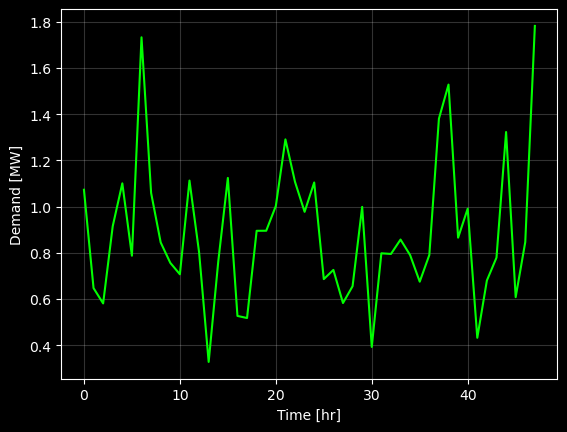
Creating the “wind” profile#
Wind speeds follow a Weibull distribution
\(f(v) = \left(\frac{k}{\lambda}\right)\left(\frac{v}{\lambda}\right)^{k-1}e^{-\left(\frac{v}{\lambda}\right)^k}\)
Where \(v\) is our random variable (velocity).
[4]:
np.random.seed(123)
shape_factor = 2.5
wind_speed = np.random.weibull(a=shape_factor,size=N)

with plt.style.context('dark_background'):
    plt.plot(wind_speed, color='lime')
    plt.grid(alpha=0.2)
    plt.ylabel('Demand [MW]')
    plt.xlabel('Time [hr]')
    plt.show()
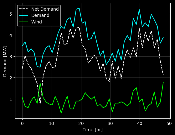
osier.CapacityExpansion will normalize the wind and solar profiles and rescale the maximum values to the rated capacity of the installed technology (for each “individual” portfolio tested). Just for fun, let’s plot the “net demand” if this wind speed were the true value.
Also note that the weibull distribution is related to wind speed, not energy production. For simplicity, we will assume they’re equal.
[5]:
with plt.style.context('dark_background'):
    plt.plot(hours, demand-wind_speed, color='white', linestyle='--', label='Net Demand')
    plt.plot(hours, demand, color='cyan', label='Demand')
    plt.plot(hours, wind_speed, color='lime', label='Wind')
    plt.grid(alpha=0.2)
    plt.ylabel('Demand [MW]')
    plt.xlabel('Time [hr]')
    plt.legend()
    plt.show()
Creating the Technology Mix#
Let’s try to meet demand with a properly sized wind turbine and storage combination.
[6]:
technologies = [lib.battery, lib.wind]
technologies
[6]:
[Battery: 815.3412599999999 MW, WindTurbine: 0.0 MW]
Setting up the Capacity Expansion Problem#
osier.CapacityExpansion inherits from a pymoo.Problem object. This class does not run the optimization itself, so we’ll have to add the pymoo pieces later. Before we can instantiate the problem, though, we need to define the objectives to optimize over!
Defining objectives#
osier comes with a set of predefined objectives, such as cost and carbon emissions. Let’s start with cost.
[7]:
from osier import total_cost
[8]:
problem = CapacityExpansion(technology_list = [lib.natural_gas, lib.battery],
                            demand=demand*MW,
                            objectives = [total_cost],
                            solver=solver)  # the objectives must be passed as a LIST of functions!
Setting up a Pymoo algorithm#
Pymoo might seem intimidating, but it too requires only a few fundamental pieces
An algorithm object (imported from Pymoo)
A problem to optimize (we created this in the previous cell!)
A stopping criterion.
[9]:
algorithm = NSGA2(pop_size=20)

import time
start = time.perf_counter()
res = minimize(problem,
               algorithm,
               termination=('n_gen', 10),
               seed=1,
               save_history=True,
               verbose=True)
end = time.perf_counter()
print(f"The simulation took {(end-start)/60:.3f} minutes.")
==========================================================
n_gen  |  n_eval  | n_nds  |      eps      |   indicator
==========================================================
     1 |       20 |      1 |             - |             -
     2 |       40 |      1 |  0.0515267085 |         ideal
     3 |       60 |      1 |  0.000000E+00 |             f
     4 |       80 |      1 |  0.0086827427 |         ideal
     5 |      100 |      1 |  0.0232186705 |         ideal
     6 |      120 |      1 |  0.0093040149 |         ideal
     7 |      140 |      1 |  0.0041260151 |         ideal
     8 |      160 |      1 |  0.0027592007 |         ideal
     9 |      180 |      1 |  0.0032212526 |         ideal
    10 |      200 |      1 |  0.000000E+00 |             f
The simulation took 3.759 minutes.
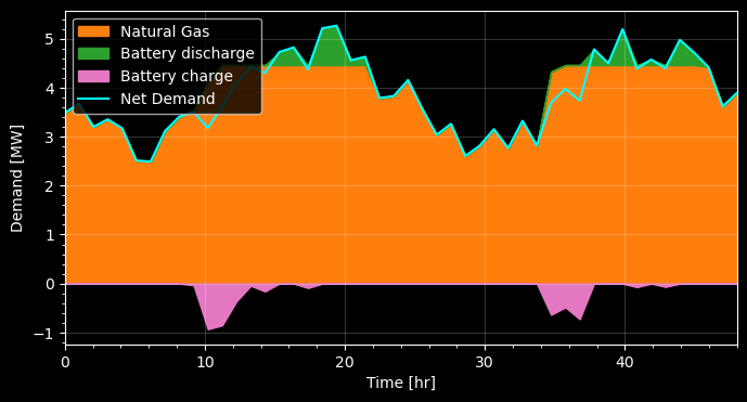
Checking the results#
We can check the results by printing the results from the res object. The res object has two variables: res.F, which contains the objective function results, and res.X which contains the corresponding energy system portfolios.
Seeing how the dispatch model uses each of the specified technologies can be useful for debugging purposes.
[9]:
display(res.F, res.X)
array([0.26311183])
array([0.84733418, 0.17653586])
[10]:
from osier import DispatchModel
lib.battery.capacity =  res.X[1]*demand.max()*MW
lib.natural_gas.capacity = res.X[0]*demand.max()*MW

technologies = [lib.natural_gas, lib.battery]
display(technologies)

model = DispatchModel(technology_list=technologies,
                      net_demand=demand)
model.solve(solver=solver)
[NaturalGas_Conv: 4.459169645008025 MW, Battery: 0.9290353002984896 MW]
[11]:
with plt.style.context("dark_background"):
    fig, ax = plt.subplots(figsize=(8,4))
    ax.grid(alpha=0.2)
    ax.minorticks_on()
    ax.fill_between(hours,
                    y1=0,
                    y2=model.results['NaturalGas_Conv'].values,
                    color='tab:orange',
                    label='Natural Gas')
    ax.fill_between(hours,
                    y1=model.results['NaturalGas_Conv'].values,
                    y2=model.results['Battery'].values+model.results['NaturalGas_Conv'].values,
                    color='tab:green',
                    label='Battery discharge')
    ax.fill_between(hours,
                    y1=0,
                    y2=model.results['Battery_charge'].values,
                    color='tab:pink',
                    label='Battery charge')
    ax.plot(hours, model.net_demand, color='cyan', label='Net Demand')
    ax.set_xlim(0,48)
    # ax.set_ylim(0,5.5)
    ax.legend(loc='upper left')
    ax.set_ylabel("Demand [MW]")
    ax.set_xlabel("Time [hr]")
    plt.show()
Adding renewable energy to a model#
The previous model used natural gas and batteries to meet demand. What if we wanted to include wind as well?
By default, the capacity expansion model samples a set of values, \(\mathcal{X}_i\), between 0 and 1 (inclusive), for each technology in the technology list where \(\mathcal{X}\) represents a fraction of the maximum energy demand (up to 100%). The capacity of each technology is calculated by
\(\mathcal{C}_i = \mathcal{X}_i\cdot \max\left(\mathcal{E}\right)\)
where \(\mathcal{E}\) is the energy demand time series.
Therefore, the maximum possible capacity for any technology is equal to the maximum demand energy demand. This is fine for dispatchable technologies because we can always choose to turn a dispatchable technology on or off. This is not true for variable renewable energy sources, such as wind. If we only built enough wind turbine capacity to match the peak demand value we
cannot be sure that the peak production will align with peak demand and
it is extremely unlikely that peak production will be sustained for any amount of time.
To get around this, we can specify a peak value greater than one. This value can be as high as you want – but best results are usually found when the maximum capacity for a renewable source is
\(\max\left(\mathcal{X}\right) = \frac{1}{CF}\),
where \(CF\) is the average capacity factor.
[12]:
problem = CapacityExpansion(technology_list = [lib.wind, lib.battery],
                            demand=demand*MW,
                            wind=wind_speed,
                            upper_bound= 1 / lib.wind.capacity_credit,
                            objectives = [total_cost],
                            solver=solver)  # the objectives must be passed as a LIST of functions!
[13]:
algorithm = NSGA2(pop_size=20)

import time
start = time.perf_counter()
res = minimize(problem,
               algorithm,
               termination=('n_gen', 10),
               seed=1,
               save_history=True,
               verbose=True)
end = time.perf_counter()
print(f"The simulation took {(end-start)/60:.3f} minutes.")
==========================================================
n_gen  |  n_eval  | n_nds  |      eps      |   indicator
==========================================================
     1 |       20 |      1 |             - |             -
     2 |       40 |      1 |  0.000000E+00 |             f
     3 |       60 |      1 |  0.0731198079 |         ideal
     4 |       80 |      1 |  0.000000E+00 |             f
     5 |      100 |      1 |  0.0023483206 |             f
     6 |      120 |      1 |  0.0255449274 |         ideal
     7 |      140 |      1 |  0.000000E+00 |             f
     8 |      160 |      1 |  0.000000E+00 |             f
     9 |      180 |      1 |  0.000000E+00 |             f
    10 |      200 |      1 |  0.0002146070 |             f
The simulation took 2.740 minutes.
[14]:
technologies = []
for X,tech in zip(res.X,problem.technology_list):
    tech.capacity = X*problem.max_demand
    technologies.append(tech)
display(technologies)
# normalize the wind speed
wind_speed = (wind_speed / wind_speed.max()) * res.X[0]*problem.max_demand
net_dem = demand*MW - wind_speed
display(f"Max wind production: {wind_speed.max()}")

model = DispatchModel(technology_list=[technologies[1]],
                      net_demand=net_dem)
model.solve(solver=solver)
[WindTurbine: 10.135967781702929 MW, Battery: 2.7950442069865686 MW]
'Max wind production: 10.135967781702929 MW'
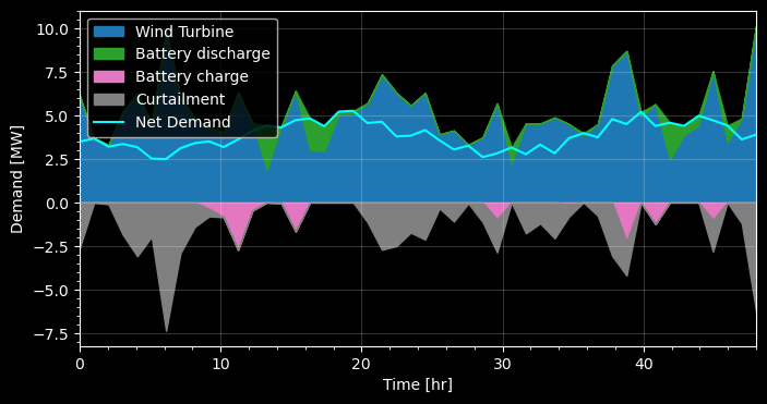
[15]:
with plt.style.context("dark_background"):
    fig, ax = plt.subplots(figsize=(8,4))
    ax.grid(alpha=0.2)
    ax.minorticks_on()
    ax.fill_between(hours,
                    y1=0,
                    y2=np.array(wind_speed),
                    color='tab:blue',
                    label='Wind Turbine')
    ax.fill_between(hours,
                    y1=np.array(wind_speed),
                    y2=model.results['Battery'].values+np.array(wind_speed),
                    color='tab:green',
                    label='Battery discharge')
    ax.fill_between(hours,
                    y1=0,
                    y2=model.results['Battery_charge'].values,
                    color='tab:pink',
                    label='Battery charge')
    ax.fill_between(hours,
                    y1=model.results['Battery_charge'].values,
                    y2=model.results['Battery_charge'].values+model.results['Curtailment'].values,
                    color='gray',
                    label='Curtailment')
    ax.plot(hours, demand, color='cyan', label='Net Demand')
    ax.set_xlim(0,48)
    # ax.set_ylim(0,5.5)
    ax.legend(loc='upper left')
    ax.set_ylabel("Demand [MW]")
    ax.set_xlabel("Time [hr]")
    plt.show()
Multiple Objectives#
What if we want to examine multiple objectives?
We simply have to import the objective we want and add it to the list! Let’s checkout lifecycle CO \(_2\) emissions.
[16]:
from osier import annual_emission

# the default emission is `lifecycle_co2_rate`
[17]:
problem = CapacityExpansion(technology_list = [lib.wind, lib.natural_gas, lib.battery],
                            demand=demand*MW,
                            wind=wind_speed,
                            upper_bound= 1 / lib.wind.capacity_credit,
                            objectives = [total_cost, annual_emission],
                            solver=solver)  # the objectives must be passed as a LIST of functions!
[18]:
algorithm = NSGA2(pop_size=20)

import time
start = time.perf_counter()
res = minimize(problem,
               algorithm,
               termination=('n_gen', 10),
               seed=1,
               save_history=True,
               verbose=True)
end = time.perf_counter()
print(f"The simulation took {(end-start)/60:.3f} minutes.")
==========================================================
n_gen  |  n_eval  | n_nds  |      eps      |   indicator
==========================================================
     1 |       20 |      6 |             - |             -
     2 |       40 |      4 |  0.0158631600 |         nadir
     3 |       60 |      6 |  0.0046803095 |         nadir
     4 |       80 |     13 |  0.0075483249 |         ideal
     5 |      100 |     11 |  0.0286189133 |         ideal
     6 |      120 |     16 |  0.0143108618 |             f
     7 |      140 |     19 |  0.0038096293 |         ideal
     8 |      160 |     20 |  0.0123935101 |             f
     9 |      180 |     20 |  0.0034209964 |             f
    10 |      200 |     20 |  0.0058865852 |         nadir
The simulation took 4.102 minutes.
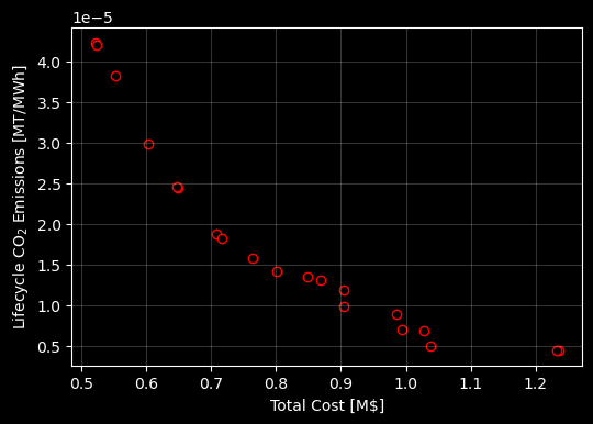
Visualizing Multi-objective Results#
Rather than identifying a single solution, a multi-objective problem generates a set of co-optimal solutions. Rather than showing the optimal dispatch results, let’s look the the Pareto front.
Objective Results#
[19]:
display(res.F)
array([[5.20590010e-01, 4.22836310e-05],
       [1.23679702e+00, 4.51507227e-06],
       [6.03522552e-01, 2.98494026e-05],
       [5.51811737e-01, 3.81846077e-05],
       [1.23258101e+00, 4.54359623e-06],
       [1.03741440e+00, 5.01230981e-06],
       [7.08193933e-01, 1.88392323e-05],
       [6.48881008e-01, 2.44276338e-05],
       [7.63720969e-01, 1.58503836e-05],
       [6.46407413e-01, 2.45709127e-05],
       [9.84786540e-01, 8.96392716e-06],
       [9.04653983e-01, 9.91760497e-06],
       [8.01539644e-01, 1.42117555e-05],
       [7.16559414e-01, 1.82649084e-05],
       [9.03588106e-01, 1.18543737e-05],
       [8.68432800e-01, 1.31478267e-05],
       [9.93427512e-01, 7.06494072e-06],
       [1.02831579e+00, 6.87727034e-06],
       [8.48928279e-01, 1.35553105e-05],
       [5.23407779e-01, 4.19378637e-05]])
[20]:
with plt.style.context('dark_background'):
    fig, ax = plt.subplots(1,1,figsize=(6,4))

    ax.scatter(res.F[:,0], res.F[:,1], edgecolors='red', facecolors='k')
    ax.set_ylabel(r"Lifecycle CO$_2$ Emissions [MT/MWh]")
    ax.set_xlabel(r"Total Cost [M\$]")
    ax.grid(alpha=0.2)

    plt.show()
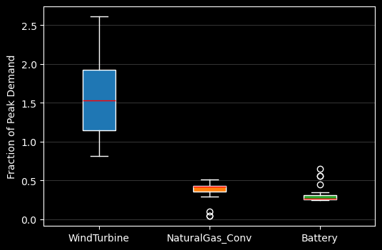
Design Results#
Below is a boxplot showing the range of values for each technology in the simulation.
Boxplots are not the best way to visualize these results, but they are the simplest.
Since we used boxplots, we lose information about which combination of technologies corresponds to each solution in the objective plot, above.
The spread of these values can suggest a degree of certainty about the level of capacity needed to meet demand while minimizing cost and emissions. We can see a huge spread in wind energy and very small spreads for natural gas and batteries. This indicates a no-lose scenario for pursuing the latter two technologies, while addressing the question about the amount of wind capacity necessary to meet demand is a lot less clear.
[21]:
display(res.X)
array([[0.81401452, 0.41946283, 0.30094145],
       [2.57475748, 0.04144996, 0.65208901],
       [1.03900939, 0.41959028, 0.24995194],
       [0.88775931, 0.45133809, 0.26573897],
       [2.61198667, 0.04144996, 0.55710663],
       [2.11218424, 0.09849739, 0.56117257],
       [1.30377163, 0.39488571, 0.25098929],
       [1.14168868, 0.42652716, 0.25387131],
       [1.42508911, 0.41533998, 0.24747279],
       [1.13773886, 0.42652716, 0.24995194],
       [1.88970608, 0.50711056, 0.25422291],
       [1.77838968, 0.37767   , 0.2562746 ],
       [1.49752492, 0.40126517, 0.29974379],
       [1.32367483, 0.39488571, 0.25098929],
       [1.67078421, 0.47594797, 0.34616406],
       [1.5663502 , 0.42795912, 0.44770924],
       [2.03385808, 0.29352286, 0.26963251],
       [2.11218424, 0.30329813, 0.26637353],
       [1.56593795, 0.50884959, 0.25559555],
       [0.82023035, 0.42580387, 0.29455337]])
[22]:
from osier import get_tech_names
with plt.style.context('dark_background'):
    fig, ax = plt.subplots(1,1,figsize=(6,4))

    bplot = ax.boxplot(res.X,
                       patch_artist=True,
                       tick_labels=get_tech_names(problem.technology_list))
    ax.set_ylabel("Fraction of Peak Demand")

    # fill with colors
    colors = ['tab:blue', 'tab:orange', 'tab:green']
    for patch, color in zip(bplot['boxes'], colors):
        patch.set_facecolor(color)

    for median in bplot['medians']:
        median.set_color('red')

    ax.yaxis.grid(True, alpha=0.2)
    plt.show()
/var/folders/6h/g412p7x53jbcqr_x5sy9z8th0000gn/T/ipykernel_47139/1527621391.py:5: MatplotlibDeprecationWarning: The 'labels' parameter of boxplot() has been renamed 'tick_labels' since Matplotlib 3.9; support for the old name will be dropped in 3.11.
  bplot = ax.boxplot(res.X,
Correlation between Wind Turbines and Natural Gas#
Perhaps we can glean more information by examining the correlation between wind and natural gas.
[23]:
with plt.style.context('dark_background'):
    fig, ax = plt.subplots(1,1,figsize=(6,4))

    ax.scatter(res.X[:,0], res.X[:,1], edgecolors='yellow', facecolors='k')
    ax.set_ylabel(r"Natural Gas")
    ax.set_xlabel(r"Wind Turbines")
    ax.set_title("Fraction of Peak Demand")
    ax.grid(alpha=0.2)

    plt.show()
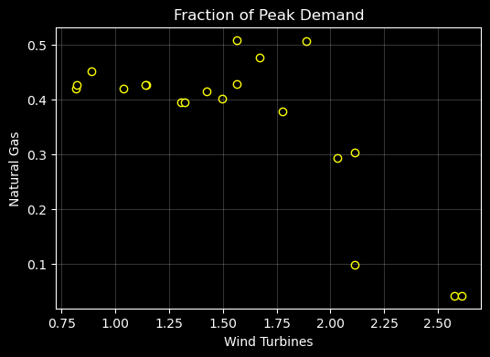
Interestingly, the capacity for natural gas is fairly stable while the capacity for wind turbines is less than double the peak demand. But the natural gas capacity drops off quickly once the wind turbine capacity exceeds twice the peak demand.